Effect of orbit precision on ERS Sea State Bias models

This page presents the results of a small study into the possible aliasing of orbit errors into parameters of sea state bias models correcting ERS-1 and ERS-2 altimeter range measurements depending on sea state and wind speed.

The data

The results obtained here are based on the latest Version 6 Ocean Product (OPR) provided by CERSAT. Corrections include (corrections in bold face are not provided on the OPR data sets):

Time tag correction of -1.5 and -1.3 ms for ERS-1 and ERS-2, respectively
GFZ/D-PAF PGM055 or DUT/DEOS DGM-E04 precise orbits
Radiometer wet tropospheric correction
ECMWF Dry tropospheric and Bent ionospheric corrections
Gaspar and Ogor [1996] Sea state bias corrections:
SSB(ERS-1)=SWH(-0.047 - 0.0035 U + 0.000160 U²)
SSB(ERS-2)=SWH(-0.048 - 0.0026 U + 0.000126 U²)
Grenoble FES95.2.1 ocean tide and loading
Solid earth and pole tide
OSUMSS95 mean sea surface

After editing all measurements are converted to single-satellite crossover height differences spanning the period of 20 June 1995 till 2 June 1996 and with a maximum time interval of 17.5 days between ascending and descending tracks.

The approach

From this data we estimate the coefficient b in the simple BM1-type sea state bias model in addition to the models given above:

SSB = b * SWH

In fact, we have enhanced this model by estimating one coefficient b_i for each SWH interval of 1 meter. Assuming the crossover height differences are due to errors in the b_i coefficients, this leads to observation equations:

Crossover difference = SSH₁ - SSH₂ = SSB₁ - SSB₂ = b_i * SWH₁ - b_j* SWH₂

The coefficients b_i (i=1...8) are solved for in a least squares minimisation of all crossover height differences.

The two alternative orbit solutions have fairly different radial precision (GFZ/D-PAF approximately 6-7 cm and DUT/DEOS approximately 4-5 cm) and differ radially by about 5 cm rms. This provides the opportunity to test the effect of orbit errors on the sea state bias estimation. At the same time, we can validate the original Gaspar and Ogor [1996] BM3-type model.

The results

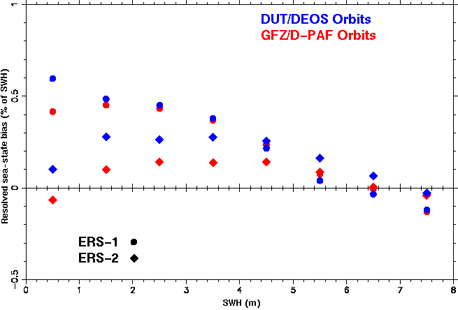
The table below lists the b_i coefficients (in percents) obtained from the analysis of the crossover height differences, for ERS-1 and ERS-2 and based on DUT and GFZ orbits. The one-but-last line gives the effect of the corrections to the SSB model: the variance of the changes to the derived sea height implied by these corrections. The bottom line gives the overall value in case only one b coefficient was estimated, as in a true BM1 model.

SWH	ERS-1			ERS-2
(m)	number	DUT	GFZ	number	DUT	GFZ
0-1	90709	0.595	0.415	42695	0.103	-0.066
1-2	254463	0.484	0.450	198712	0.278	0.099
2-3	215105	0.450	0.432	207745	0.263	0.141
3-4	115812	0.380	0.368	122849	0.276	0.137
4-5	52027	0.216	0.237	62725	0.256	0.141
5-6	20668	0.040	-0.006	28233	0.162	0.086
6-7	7343	-0.033	-0.130	11542	0.065	0.003
7-8	2471	-0.119	-0.227	4307	-0.117	-0.040
Var (cm²)		0.376	0.352		0.192	0.050
0-8	758598	0.370	0.355	678808	0.244	0.118

The values are presented in graphical form below. Circles are for ERS-1, diamonds for ERS-2. Blue (light grey) markers are for DUT orbits, red (dark grey) markers for GFZ orbits.

The conclusions

The adjustments to the Gaspar and Ogor sea state bias models are of the order of 0.2 to 0.4% of SWH and would result in a 0.05 to 0.38 cm² correction to the sea surface height. Naturally, the adjustments do not include effects of windspeed, but results show a clear tendency that the current sea state bias is underestimated for the range of 1-5 meters of SWH.
Both the trend of the SSB as a function of SWH and the overall implied variance are similar to the differences found between a BM3 and BM4 model. Yet, the variances appear too small to warrent the selection of a BM4 over a BM3 model.
Remarkably, the selection of the orbit (DUT or GFZ) does have little effect on the ERS-1 sea state bias adjustments, but certainly has a considerable impact on the ERS-2 results. In the later case the estimated adjustments are about 0.1% for SWH up to 5 meter.
The effect of orbit error on the SSB coefficient also urge for caution in generating SSB models and prevailing one over the other. The SSB estimation still is quite sensitive to many external effects.

Acknowledgements

Thanks to Philippe Gaspar for his comments.

Questions or comments:

Remko Scharroo, remko.scharroo@lr.tudelft.nl.

20 May 1997.